The commercial property insurance industry has become increasingly
alarmed over the risks involved in insuring business interruption.
Business interruption coverage is designed to cover the foregone
profits and extra expense incurred following an insured loss.
Coverage is provided until the insured has recovered to pre-loss
levels, thus a BI loss could potentially go on for years. Due
to business reengineering practices such as "just-in-time,"
the potential exposure has grown substantially in recent years.
A recent example is a large Japanese automaker, which had a loss
in Feb. 1997 estimated to be in the neighborhood of $320 million.
Decreased inventory levels, sole-sourcing, and reduced make-up
capacity are a few of the risk factors which have been accentuated
by just-in-time changes. Complex interdependencies between various
locations within companies produce a "ripple effect"
when a loss occurs. When a loss does occur, a company will attempt
to minimize the effect of the loss, including shifting manufacturing
to the products with the highest profit margins (when this is
prudent) and buying materials on the market to honor sales contracts.
The business interruption loss is calculated as the lost profits
which would have been made, according to forecasted sales, as
well as any extra expense involved in trying to mitigate the effect
of the original loss, up until the time at which the company has
rebuilt the capacity to sell at the forecasted levels.
It is perhaps not surprising then, after taking all of these factors
into account, that the commercial property insurance industry
has not had a good method of predicting the expected BI loss in
the past. To determine the expected BI loss, one would
also need to have accurate estimation of probabilities associated
with the frequency and severity of losses as well as downtimes
and recovery periods following a loss. Often the underwriter will
investigate the Maximum Foreseeable Loss scenario, that
is, a "worst case" scenario, which is in fact not the
absolute worst case in which everything is lost, but rather a
scenario which is assumed to only occur if all protection systems
fail - generally a loss whose probability of occurrence is quite
small, usually .01 or less on an annual basis. These MFL studies
are fine, except that they only represent one point in the whole
probability distribution of BI losses. After the MFL study, the
mathematical basis for pricing insurance rates falls apart considerably,
with one perhaps taking a small fraction of this MFL as the desired
premium, with no appeal to the actual probability distribution
involved.
A Systems Dynamics Approach
In order to develop a better model, a natural approach is to try
to build a model which would simulate the same processes that
are used when evaluating a BI loss, in order to estimate the
probability distribution of BI loss. That is, a model of the company
is built which simulates product flow or cash flow, taking into
account inventory levels (if they even exist after just-in-time
practices have taken their toll,) interdependencies between locations,
make-up capacity, seasonal demand, and market share. Once a working
model has been built and validated, losses may be introduced at
various locations, each loss having its own probability distribution
for frequency and severity of loss, length of downtime (the time
period during which no recovery can be made) and recovery period.
The resulting BI loss is then calculated for each loss scenario.
Typically, thousands of scenarios must be made in order to simulate
over the whole range of the distributions involved. The simulated
BI losses can then be examined to get an idea of the overall shape
of the BI probability distribution (this same idea has been explored
independently (Arthur, 1996.)) The incorporation of probability
distributions as well as the focus on developing an "accurate"
model for the flows, makes this application of systems dynamics
different from applications where the emphasis is on the power
of the model as a decision-making tool (Forrester, 1961.)
An Example
The following example is real, and concerns a nationwide product
distribution system. Although the system is relatively simple
in comparison with other possible systems, the data was available,
and the customer had a potentially large BI risk which was not
felt to be well understood, so it was a good candidate for the
model. There are five main distribution centers in the USA, at
which the product flows in and is sent to its destination by way
of a vast network of handling centers and trucking operations.
There is no transfer of product between the five centers, thus
no interdependency. If one center should become
inoperable, the other centers could accommodate the added demand
and would eventually take up the overflow by hiring more workers.
Even if the largest center were to go down, there would be an
initial loss of profits from inability to deliver the product,
but after the third week all of the product would be distributed,
hence most of the BI cost would be in the form of extra expense
due to new hires and overtime. Due to the vastness of the trucking
and handling operations, it was not felt necessary to include
these smaller facilities in the model. The
market is very fickle, as prices are competitive, hence market
share represents an important feedback mechanism in the model.
Following a major loss, an advertising campaign would begin, in
order to gain back lost market share, and the model allows for
this effect of advertising.
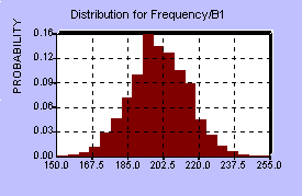
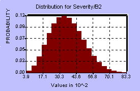
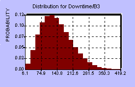
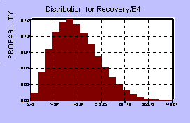
To asses the probability distributions involved, the MFL study provided a benchmark, that is, one point on the BI distribution, and some assumptions had to be made about the actual shapes of the various distributions at each center. It should be mentioned that these assumptions, perhaps more than anything else, can have a dramatic influence on the resulting BI distribution. Each center has four distributions associated with it, so in all there were 20 probability distributions involved. The five centers were assumed to behave independently of each other, since they are spread out across the country, however there is probably some weak dependence, since the overflow from one center could increase demands on the other centers and affect their distributions as well. Below are diagrams of the distributions for the first center and the distribution for BI resulting from the model.
Center A:
Frequency of Loss (years between losses) Severity of Loss (% of sorting capacity lost)


Downtime (days) Recovery Period (days)
Twenty such distributions were used as random inputs into the
model, and the resulting BI computed over many simulations. The
shape of the BI distribution appears below.
Conclusion
Once a convincing prototype model was initially completed, the
next objective was to work with a few specific customers, collect
the data, and try to then determine a general approach to determine
the BI risk for all customers. The quest for product-line data
has been frustrating, since many companies think in terms of net
sales rather than net production, and hence do not keep track
of this data. In the example above, product-line data was publicly
available, but still did not differentiate by type of product,
hence it represents more of an average product flow. Efforts in
collecting financial flow data have been more fruitful, but still
require diligent investigation with regard to interdependency
flows and make-up capacities. Another problem exists in that companies
are subject to change, so that the original model must be continually
updated by someone competent in using systems dynamics software.
Because companies typically do not try to estimate probabilities
of losses, they often have no clue of how likely a particular
scenario is, nor how they would specifically cope with such loss
scenarios, thus it is difficult to get a good idea about the loss
distributions involved. Because of the amount of time required
to collect data, create a model, and keep it up to date, this
particular approach does not seem to be a feasible option for
all of our customers at this time. It may be more reasonable to
try to develop a less sophisticated model which would apply to
most customers, using financial information, while developing
sophisticated systems dynamics models for the customers who pose
the highest potential risk. The process of data collection in
itself has proved to be an enlightening experience for the customer
as well as the insurer, and questions relating to interdependency,
make-up capacity, seasonality, and likelihood of loss will continue
to be part of the service to our customers.
References
Arthur, W.B., Eberlein, R.L., 1996, Sensitivity Simulations, Proceedings of the 1996 International Systems Dynamics Conference, Vol. 1, P. 44, Cambridge, MA
Forrester, J. W., Industrial Dynamics, 1961, MIT Press, Cambridge, MA