Abstract: In this study, we present crisp and fuzzy nonlinear simulation models which are represented by nonlinear differential equations. First, we consider dynamical properties of some chaotic systems such as Van der Pol and Lorenz equations. Then stability, nonlinear stability, unstable node, chaotic phenomena, bifurcation and catastrophic behaviours of the lake pollution, predator-prey models, spread of aids, Zeeman's models for the heartbeat, inverted pendulum and Richardson's "arms race" have been solved by numerical solution with MATLAB.

Introduction:Recently, (crisp) nonlinear and fuzzy dynamical systems have become a popular research in the physical, technological /engineering and social processes or systems . The analysis of physical systems involves two steps:

a)Developing models for physical systems which accurately represent their physical behaviour, b)Predicting the behavior of systems based on these models1. Theories of nonlinear dynamics focused on two and three variable systems and their limit cycles. The rapid rise in the last decade, of chaos theory has had some important positive messages for us.

Definitions: Nonlinearity : Nonlinear functions may arise in a dynamical model either because they are intrinsic to the nature of the system or because , in a technological case such as a control system, they have been deliberately introduced by the designer for a specific purpose2. Nonlinear dynamical systems have some interesting properties: their behavior in the limit reaches a steady state (fixed point), an oscillation(limit cycle), or an aperiodic instability(chaos)3.

Stability (The Lyapunov criterion) states that, if the origin is a singular point, then it is stable if a Lyapunov function V(x) can be found with the following properties:

a) V(x) 0 for all values of x 0, b) dV/dt 0 for all x , for continuos system , or V X(k) V X(k+1) - V X(k) 0, for all x , for discrete time systems4.

Chaotic Systems : Let V be a set. f : V V is said to be chaotic on V if ;

1. f has sensitive dependence on initial conditions. 2. f is topologically transitive. 3. Periodic points are dense in V. A chaotic map posseses three ingradients: Unpredictability, indecomposability, and an element of regularity. A chaotic system is unpredictable because of the sensitive dependence on initial conditions. It can not be broken down or decomposed into two subsystem(two invariant open subsets) which do not interact under f because of topological transitivity, and in the midst of this random behavior, we neverthless have an element of regularity, namely the periodic points which are dense5.

Limit Cycles:A distinctive characteristic of nonlinear systems is the possibility of exhibiting limit cycles. A limit cycle is one for which trajectories slightly perturbed from it are attracted back to it. An unstable limit cycle is one for which perturbed trajectories do not return to it6.

Bifurcation Condition: It has been investigated that if a nonlinear differential equation discretized and approximated by a difference equation, chaotic behaviour and bifurcation may occur and special attention must be paid when a nonlinear differential equation is discretized by using the forward Euler Method7.

Fuzzy Dynamical System(FDS): The expilicit dependence of a dynamical system on time and initial condition is desirable in stability and optimization investigations. It occurs in the attainability sets of crisp dynamical systems. This suggests that fuzzy dynamical systems be defined in terms of attainability sets. To this end, a fuzzy dynamic system(FDS) on a state space X is defined here axiomatically in terms of a fuzzy attainability set mapping f: X x TS satisfying the following four axioms:

(A) f(x,t) is defined for all (x,t) X x T ; (B) F(x,0) = X_x for all x X ;

(C) F(x,s+t)=F(F(x,s),t) for all x X and s,t T; (D) F is jointly continuous in (x, t) 8. In physical systems, it is sometimes difficult to describe a complex system using the linearization or identification techniques. Tagagi and Sugeno used fuzzy implications to express a complex system which is called the fuzzy model. In general, the construction of the fuzzy model is based on the physical properties of the system, the input-output data, and the corresponding empirical knowledge and so on. The main advantages of fuzzy control are: (1) no mathematical formulation of the system is needed. (2) Linguistic variable and approximate reasoning are used to describe the inexact objects and achieve multiobjective control9.

3. Examples of Some Physical Processes and Solutions

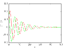
3.1. Rayhleigh's VAN der POL Equations

Van der Po l 's differential equation is x" + ( x ' ² -1) x ' + x = 0 . A feature of the solutions is the presence of limit cycles. Find these, and investigate their stability. Try graphing x as a function of the time when is equal to one or more [10].

The equations become x₁' = x₂ , x₂' =- x₁ + (x₂ -x₂³ ) . Solutions :

Figure 3.1.a. The case for = - 0.19 is stable. Figure 3.1.b. The case for = 20 is unstable.

3.2. LORENZ Equation

The equations Lorenz considered were the following :

dx/dt = - x + y , dy/d t = - x z+r x - y , dz/dt= x y - b z

where, , r and b are dimensionless parameters. The quantity x is proportional to the circulatory fluid flow velocity, y characterizes the temperature difference between rising (and falling fluid regions and z character) the distortion of the vertical temperature profile from its linear with heigh equilibrium variation [11]. Solutions:

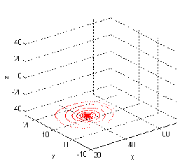
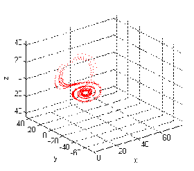
Figure 3.2.a. The case for b=8/3,=10,r=28 is chaotic. Figure 3.2.b. The case for b=8/3,=20,r=25 is bifurcation.

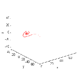
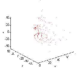
Figure 3.2.c. The case for b=2.67,=20,r=15 is bifurcation. Figure 3.2.d. The case for b=2.6,=65,r=42 is unstable.

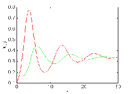
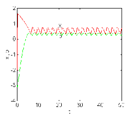
3.3. LAKE POLLUTION Equation

Three components are involved in the model. x is the total biomass of all algal species;y is the soluble phosphate concentration of Anabaena,one of the phytoplank-ton genera; x satisfies a generalized logistic equation; as x increases the growth rate decreases.The death rate is proportional to z .The equations are: dx/dt= -c₁x³+c₂xy-c₃ z and for the phosphates dy/dt= -c₄(y -a₀) . where a₀ is the equilibrium concentration. dz/dt = c₅ yz - c₆ xz these are the three equations of the model[10]. Solutions :

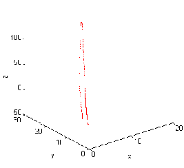
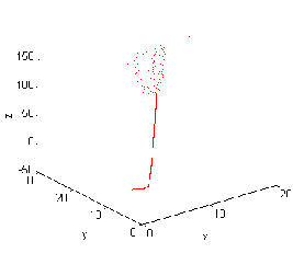
Figure 3.3.a. The case for c₁ = -10 , c₂ = 0.6, c₃ = 0.05 , Figure 3.3.b. The case for c₁ = -15 ,c₂ = 0.1, c₃ =- 0.55 ,

c₄ =1,c₅=1.35,c₆=1.95 is c₄ = -1 stable. c₅=0.35 , c₆=0 . 1 is bifurcation.

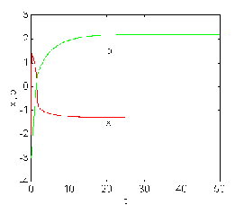
3.4. The Predator-Prey Model with INTERNAL COMPETITION

Population growth is often replaced by the logistic equation dx/dt=ax-ex². If a population is growing according to this equation, it will approach the value x_a=a/e asymptotically from below. This value would represent the greatest population that the environment can support. So if the two species are competing internally for resources , space , etc. The equations become dx/dt=ax-bxy-ex²,dy/dt= -cy+dxy-fy²[10].Solutions:

Figure 3.4.a. The case for a = 1.625 , b=4.2,c = 0.29 , Figure 3.4.b. The case for a = 0.25 , b=0.42 , c = 0.29 ,

d=0.904 , e=0.642 , f=0.061 is stable . d=0.50 , e=0.60 , f=0.06 is unstable .

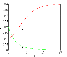
3.5. The Initial SPREAD OF AIDS

This model is just concerned with the initial spreading of the disease. First, consider just the spread through sexual contact. Suppose that at time t there are in a group of inviduals p₁ homosexual males of which x₁(t) are infected, p₂ bisexual males of which x₂ (t) are infected, heterosexual females of which y(t) are infected, and r heterosexual males of which z(t) are infected. Assuming that the rate of infection is proportional to the number of contacts, and neglecting "removals", the following system results: x₁'=a₁x₁(p₁-x₁)+a₂x₂(p₁-x₁) , x₂'=b₁x₁(p₂-x₂)+b₂x₂(p₂-x₂)+b₃y(p₂-x₂)

y ' = c₁ x₂ (q - y) + c₂ z (q - y) , z ' = d₁ y (r - z) [10]. Solutions :

Figure 3.5.a. The case for a₁ =-5,a₂=5,b₁ =5,p₁ =1.01, p₂ =0.99, Figure 3.5.b. The case for a₁ =-4,a₂=5,b₁ =.1,p₁ =1.1, p₂ =0.5,

b₂ =1.01,b₃ =0.99,c₁ =1,c₂ =1,q=1,d₁ =1.1,r =0.99 is stable. b₂ =1.9,b₃ =.2,c₁ =.5,c₂ =1.5,q=1.5,d₁ =1.3,r =1.3 is unstable.

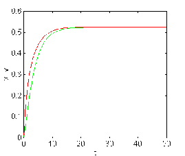
3.6. Zeeman's Model For The HEARTBEAT

There are two dependent variables in the model: x refers to muscle fiber length, and b refers to the electrochemical activity. The values for diastole(relaxed equilibrium) will be x₀ , b₀ , and those for systole(concentrated state) will be x₁ , b₁ . Each of these states is an equilibrium of the model. The main parameter will be T , which refers to the over all tension of the system.The equations for this are x'= -(x³-Tx+b),b'=x-x₁. Where is a small parameter that depends on the time scale. For numerical experiments, it will probably be sufficient to take = 0.1 . In order that the systole state should be an equilibrium[10]. Solutions :

Figure 3.6.a. The case for e =0.1,T=1,x₁ =0.57185 is stable. Figure 3.6.b. The case for e =0.1, T=0 , x₁ = -1.3 is unstable.

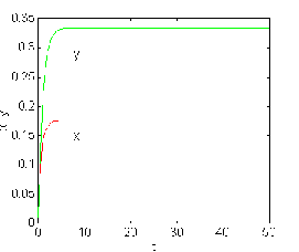
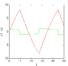
3.7. Richardson's " ARMS RACE "

To set up the model we need variables; dependent and independent. The independent variable is the time t , and we shall take the unit of time to be the year. The dependent variables will represent the expenditures x(t) and y(t) on armaments of two arms, respectively. Now consider the factors that would cause x to change. Three will contribute to the model: (1)the state of preparedness for war of the other country tend to increase x; (2) the cost of armanents will tend to decrease the rate of change of x; and (3) a sense of grievance against arm will tend to increase x . In the model, these factors are assumed to lead to the equation dx/dt=ay-mx+g . Where a,m and g are constants. In the same way, we have for against arm dy/dt=bx-ny+h [10]. Solutions :

Figure 3.7.a. The case for m=0.96,a=0.41,g=0.29,b=0.501, Figure 3.7.b. The case for m=2.5,a=3.5,g=0.325,b=0.567,

n=0.619 ,h=0.061 is stable . n=1.2 ,h=0.3 is unstable .

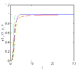
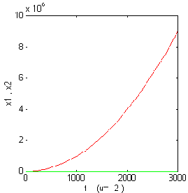
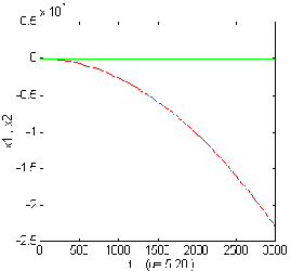
3.8. INVERTED PENDULUM SYSTEM (Crisp approach)Equation is -ml² d^2/dt2 +(mlg)Sin()=u(t). Where m is the mass of the pole located at the tip point of the pendulum, is the deviation angle from vertical in the clockwise direction, u(t) is the torque applied to the pole in the counter clockwise direction ( u(t) is the control action), t is time,and g is the gravitational acceleration constant , x₁ = deviation angle , x₂=d/dt velocity of deviation . So the equation become dx₁ /dt= x₂ , dx₂ /dt= (g / l) Sin(x₁) - (1/ml²) u(t) [12]. Solutions :

Figure 3.8.a.The variation of x_{1 ,}x₂ for u= -2 . Figure 3.8.b. The variation of x_{1 ,}x₂ for u= 5.28.

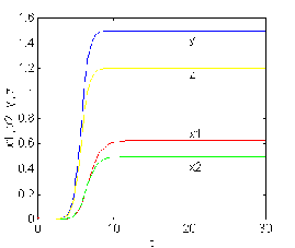
3.9. INVERTED PENDULUM SYSTEM(Fuzzy approach)

We want to design and analyse a fuzzy controller for the simplified version of the inverted pendulum system shown in Figure 3.8.a.and b. From differential equation describing the system we get the linearized and discrete-time state-space equations as matrix difference equations x₁ (k+1) = x₁ (k) +x₂ (k) , x₂ (k+1) = x₁(k)+x₂(k) -u(k) .

For this problem we must construct membership functions for x₁ (k) , x₂ (k) , u (k) and nine rules in a 3 x 3 FAM table. With this table our aim is to stabilize the inverted pendulum system. Using these nine rules we will then conduct a simulation. For four cycles of simulation using the matrix difference equations, above, for the discrete steps 0 k 3 . The FAM table will produce a membership function for the control action , u (k). To start the simulation we will use the following crisp initial conditions: x₀ (0)= -4 degree per second (dps) , x₁ (0)= 1^o , u (0)= -2 we assume the universe of discourse for the three variables to be -2^{o x}₁ 2^o , -5 dps x_{2 5 dps and -24 u (k) 24 . We will defuzzy the membership function for the control action using the centroid method and then use the recursive difference equations to solve for new values of x1} and x₂ 12:

for k=1, x₁ (1)= -3,x₂ (1)= -1, u (1)= -9.6 ,for k=2 , x₁(2)=-4,x₂ (2)=5.6 , u (2)= 1.6 ,

for k=3,x₁(3)=1.6, x₂(3)=1.6, u (3)=5.28 ,for k=4,x₁(4)=3.2 ,x₂ (4)=-2.08,u(1)= 1.12

4. Comparison Crisp and Fuzzy Nonlinear Models

We can point out that it is easy to divide a nonlinear system into some linearized subsystem on an input- output space. This means that the system is approximated by piecewise linear functions. Since many nonlinear systems can be approximated by piecewise linear functions, this means that it can be widely applied not only to fuzzy system, but also to nonlinear system .

5. Result

In the last decade nonlinear especially chaotic systems have been must popular research areas in physics , biology and economy from the point of view of system theory . Matching the crisp and fuzzy dynamic systems would be emerging powerful technologies / tools in order to search the stability conditions , chaotic phenomena and catastrophic behaviour.

References

1. LEITCH , R.R. ,Modelling of Complex Dynamic Systems, IEE Proceedings

Vol.134, pt.D, No 4 . July 1987, pp 245-250.

2. COOK,P.A.,Nonlinear Dynamical Systems,Prentice-Hall Int.(UK) Ltd., 1986 .

3. LIN, C.T., LEE,C.S., Neural Fuzzy Systems , Prentice Hall, N.S. ,1996 .

4. DISTEFANO,III, J.J., STUBBERUD, A.R.,WILLIAMS, I.J., Schaum's Outline of

Theory and Problems of Feedback and Control Systems, sec.Ed., Schaum's

Outline Series, McGraw-Hill, Inc., New York 1990.

5. DEVANEY, R. L., Introduction to Chaotic Dynamical Systems, Addison-Wesley

Dub.Comp.,Inc.,1987.

6. BROGAN,W.L., Modern Control Theory, Third Ed.,Prentice Hall Int., Inc.,1991 .

7. HIRAI, K.,ADACHI,T.,Chaos and Bifurcation in Numerical Computation by the

Runge-Kutta Method.,Int.J.System Sci.Vol.25,No.11,1994,pp.1695-1706.

8. KLOEDEN, P.E.,Fuzzy Dynamical Systems, Fuzzy Sets and Systems 7(1982) ,

pp.275-296.

9. CHEN ,C. L.,CHEN, P.C.,CHEN, C.K., Analysis and Design of Fuzzy Control

System,Fuzzy Sets and Systems 57 (1993) , pp.125-140.

10. DANBY, J.M.A., Computing Application to Differential Equations, Reston

Pub.Comp. , Inc., Reston , 1985.

11. OTT, E . , Chaos in Dynamical Systems , Cambridge University Press , 1993 .

12. ROSS,T.,Fuzzy Logic with Engineering Applications,McGraw-Hill,Inc.,

NewYork, 1995.

ISDC '97 CD Sponsor